Text-to-SQL with LLMs: why your AI agent needs a semantic layer

Tue Aug 18 2026

Technology

SQL

Topic

Analytics Engineering

Data Platforms

AI analytics runs on the same principle that made BI reliable: give the tool the right context about your data. Skip that step, and the cost is concrete for data and analytics leaders: no AI adoption in analytics means the same old speed of work; On the other hand, the wrong implementation means analysts' time lost to debugging AI output or, even worse, steering on results that look right but lead to the wrong decisions. We tested this directly, comparing an LLM with no data context against the same model equipped with a structured context layer, specifically for text-to-SQL query generation(what the industry calls a semantic layer) built from metadata and documented data relationships. The results were unambiguous. Without context, the LLM invented table names, hallucinated column values, and produced SQL that would not run. With the context layer, it returned accurate, immediately runnable queries from the first attempt, with zero hallucinations across three distinct business questions.

The challenge that started this

I ran into this unexpectedly on a client engagement. We were helping their data analysts use LLMs to get better visibility into Databricks usage and costs. The goal was to speed up the analytics to spot inefficiencies: idle compute clusters burning budget, pipelines running for hours and wasting resources, and services nobody was actually using. Given a small analyst team and a wide adoption in the organisation with thousands of employees, we needed a reliable way to analyse records daily/weekly and act on them quickly. When I connected the LLM to the Databricks system tables, it failed immediately. The model invented tables that did not exist, guessed at column values, and produced wrong results. For a small team already stretched in its capacity, that is not a minor inconvenience but time wasted debugging AI output instead of delivering smarter with it.

The root cause was not a model limitation. The LLM simply did not know how the data was structured, so it tried to guess. In fact, I was surprised because the Databricks system table documentation is accessible online for everyone. Now, most probably you are an organisation with your own unique data, column conventions, or business logic. Every time the model guesses wrong, you pay for it: in analyst time, in misleading output your team might act on, and in compliance risk when an AI tool is reasoning about data it was never meant to see. Thus, the more complex and unique your data environment is, the harder it is for a general-purpose LLM model to navigate correctly.

The question was: what is the minimum structured context needed to fix this, and how should it be built? After reading this article, you will get all the answers.

This article has 2 parts: Part 1 explains how to do it and why to use the Context Layer; Part 2 shows the technical details and our methodology to make these results reproducible.

Part 1: Why text-to-SQL and why the context layer is the missing piece

The diagram below shows what a full conversational analytics system looks like. A user asks a natural language question; the system generates a SQL query, runs it against your data, and returns a formatted answer. Follow-up questions deepen the analysis in a continuous loop.

Conversational Analytics: The complete loop

Diagram 1: Conversational analytics architecture: text-to-SQL complete loop with context layer

Text-to-SQL sits at the heart of this loop. Get it right, and the rest of the system works. Get it wrong, and every answer the system produces is unreliable. Three reasons make it the right place to start if you need to improve your conversational analytics.

Transparent. Every query can be read and audited before it touches data. If the output looks wrong, you can trace exactly where the error occurred. No black box, making governance and continuous improvement easier.
Portable. Generating a SQL query requires only schema knowledge, not access to the actual data. If your governance policy does not allow an AI agent to execute queries autonomously or access the data itself, a human can review and run the query manually. No direct connection to production systems is needed.
Plays to the LLM's strengths. LLM’s are genuinely good at writing code. SQL doesn’t have as rich semantics as our spoken languages; thus, it makes the probabilistic nature of LLM’s a bit more predictable. Thus, given the right context, a model produces complex, multi-table SQL in seconds that would take an analyst minutes to write.

That last point is where most implementations break down, and that is exactly where the context layer comes in.

Building the right context layer

Before analysts could use a BI tool reliably, someone had to prepare the data behind it: document the tables, define the relationships, establish what each column means in business terms. That preparation is what made BI reliable. The same preparation is what makes LLM-generated SQL reliable.

The context layer is a structured package of knowledge about your data that the LLM receives alongside every question it is asked. We found out these 4 key steps:

Identify the “source-of-truth” data. That is your curated data, which you trust to base your decisions on.
Data documentation: column names, accepted values, descriptions, and any business context that explains why the data looks the way it does. This should be captured via YAML or JSON files that can provide the metadata.
Semantic Model: it maps the relationships between tables explicitly, specifying which tables can be joined and how to correctly answer the business question. This can be done using the same YAML file as well, but it doesn’t have to be.
Restrict the LLM to only these documented sources. This is the key part, as you want to prevent the LLM from using unauthorised data or non-analytics-ready data yet.

Now, we can test whether this packaged context layer produces any value compared to the baseline situation without it.

The experiment

We tested whether this context layer actually makes a difference by running the same three business questions through two versions of the same LLM:

LLM without Context: LLM has no specialised knowledge about our business problem, the data related to it, and how to correctly combine it
LLM with Context: We added our suggested context layer to provide the LLM with knowledge about our data and its documentation. In this case, it was the metadata of Databricks system tables and a semantic model showing how to join those tables correctly.

LLM without context vs. LLM with context

Diagram 2: LLM without context(left) vs LLM with semantic layer for text-to-SQL that creates an enriched context layer.

To see the full produced code, see Part 2: Technical Deep Dive.

Text-to-SQL results: LLM with context vs. without

We took three questions that product owners typically ask about their Databricks account and ran those questions via two versions of the same LLM. Both ran against live Databricks system tables in Xomnia's own workspace, which meant results were verifiable against real data. We evaluated each output on three criteria: accuracy, hallucination rate, and actionability.

Question 1: Which workspaces are running but never used?

Business question: List all the workspaces that are currently running and have never been used

Prompt: Build a table that returns all the workspaces that are running and have never been used

Analysis: The image below demonstrates some of the fixes that an analyst has to make in the very first SQL CTE to fix the wrongly generated logic.

Business question 1

Swipe left/right to see the full table →

Criteria	LLM without Context	LLM with Context
Accuracy	Critical failure Conflated event-based usage data with static workspace status. Even after manual fixes, identified only 30% of correct workspaces.	Success Correctly used DBU consumption to identify zero-cost workspaces. Ran with one minor adjustment. Also surfaced active clusters with no user activity, enabling additional analysis beyond the original question.
Hallucinations	High frequency Invented `system.workflows` (does not exist), columns `workspace_status` and `created_on` (do not exist), and filtered on "ENABLED" instead of the correct value "RUNNING".	Zero Correct schema names, column names, and accepted values throughout, without guessing.
Actionability	Negative ROI Required significant time to debug. Furthermore, the final output lacked the metadata needed to take any action.	High ROI Included `workspace_name` and direct URL for Databricks UI drill-down, plus a full activity breakdown across queries, clusters, and warehouses, enabling immediate investigation.

Conclusion: LLM with Context completely outperformed the one without Context. The baseline output consumed analyst time and still returned wrong answers. The Context output saved time and delivered something immediately usable.

Winner: LLM with Context

Question 2: costs per service across the organisation

Business Question: List the costs for each type of service used in Databricks across the entire organisation.

Prompt: Create a list that shows the costs for each type of product/service used in Databricks across the entire organisation. Some columns I want to see: cost, product_name, number of distinct users

Analysis:

Business question 2

Swipe left/right to see the full table →

Criteria	LLM without Context	LLM with Context
Accuracy	Partial High-level summary was correct, but the user counting attempt failed: over-complicated the "User Count" by attempting to correlate services to users via unnecessary joins, rather than using the simple existing table.	Solid Correct service grouping and user counts. The solution was slightly over-engineered due to joining two tables where a single table would be enough. Crucially, the logic was valid, and the output was accurate.
Hallucinations	Logic hallucinations It didn't just invent a table, but it hallucinated a relationship (join) between tables that wasn't necessary. The model guessed the wrong data structure for counting users, leading to errors. It made a good attempt, given a limited understanding of the table columns and a good "rule of thumb," but it doesn't always work.	Zero The model stuck strictly to the available schema. Furthermore, the model read and found the current struct with all the user attributes, and it produced a correct count, unlike the LLM without context.
Actionability	Low Flawed user counts made the output unreliable for business decisions to be correctly made based on this output.	Medium Correct service classification made the output interpretable. Did not automatically distinguish between All-purpose, SQL, and Jobs compute sub-costs, but the data was accurate.

Conclusion: The LLM with Context did a significantly better job of understanding the exact columns and fields across the tables, how to join them, and how to derive good, high-level metrics as requested. Furthermore, we see that context doesn't always equal "perfect insight." While the LLM with Context prevented errors and hallucinations (solving the accuracy problem), it didn't automatically make the results actionable.

Winner: LLM with Context

Question 3: auto-termination settings for compute resources

Business Question: Make a list of all the resources and their settings for auto- termination time. Furthermore, list the resources that have no auto-termination at all

Prompt: Make a list of all my resources and their settings for auto stop/auto termination, so I can prevent idle costs by looking over the settings. Finally, list only those resources that have no auto termination / have it set up for more than 45 minutes

Analysis:

Business question 3

Swipe left/right to see the full table →

Criteria	LLM without Context	LLM with Context
Accuracy	Superficial High-level cluster classification was correct, but the model missed `delete_time`, treating already-deleted clusters as currently active and flagging them as risks.	Context-aware Correctly identified `delete_time` from the schema, distinguishing historical records from running resources. The output reflected the actual current state.
Hallucinations	Column hallucinations Tried to select `start_date` (does not exist); could not resolve between `create_time` and `change_time`, guessing incorrectly.	Zero Exact column names throughout.
Actionability	Misleading The results looked actionable: listed resources with risky settings, named owners, and provided termination times. However, those resources had already been deleted. An analyst acting on this would investigate clusters that no longer existed and would waste their time.	High Surfacing `delete_time` allowed immediate verification that the flagged resources were already gone, changing the entire interpretation of the output and preventing the waste of time for an analyst.

Conclusion: This example shows the most dangerous failure mode: an output that looks correct but produces misleading results. The model without Context returned a correct list, but it had no way to know those entries were historical without schema context. By simply knowing the schema definition for deletion_time, the LLM with Context revealed that the "risky" clusters were already dead. One column in the documentation changed the entire output.

Winner: LLM with Context

What this means for your data team

The results across all three questions point to the same root cause for teams building conversational analytics: the bottleneck for LLM-based analytics is not model intelligence; it is data context. Modern LLMs can write excellent SQL. What they cannot do is infer your specific schema, understand your business naming conventions, or know which columns hold which values in your environment. A context layer addresses this directly.
The practical return is real. A model that produces runnable, accurate SQL from the first attempt saves analysts hours of debugging every week. It also eliminates a harder-to-catch class of errors: queries that execute but return wrong answers, or analyses that look actionable but send teams in the wrong direction, as we saw in questions 2 and 3. For organisations in regulated environments, there is a governance benefit too: with a context layer in place, the LLM's reasoning is traceable. You can show exactly what data it was given and why it answered the way it did.
The good news is that most teams are closer to a working context layer than they realise. If you already maintain any of the following, you have most of the raw material:
- dbt models or documented table definitions
- A Looker, Power BI, or similar semantic layer
- KPI definitions, business glossaries, or measure documentation
The additional work is structuring this for an LLM: YAML metadata files, column descriptions, relationship mapping. In a well-documented environment, it takes days, not months.
If your data already lives on Databricks or Snowflake, you may have a head start. Both platforms offer native conversational analytics tooling (Databricks Genie and Snowflake Cortex Analyst), giving your team a starting point rather than a blank page.

What this proves about context or semantic layers and AI analytics"

Data modeling for AI follows the same principle as data modeling for BI. The format is different, and the consumer is an LLM rather than an analyst, but the underlying logic is unchanged: give the tool a clean, documented, relationship-aware context of the data, and it will produce reliable output. Skip that step, and you will spend most of your time recovering from the consequences.
If you are currently building any kind of AI-powered analytics, the most useful question to ask is whether the LLM behind it has a trusted context layer or whether it is guessing at your schema from general knowledge. That question predicts the quality of your results more reliably than the model you chose or the platform you deployed it on.

Taking your context layer further

This blog covered just the foundations of building the context layer. For more advanced teams and use cases, the following components will improve how well the LLM understands your data and your users' questions. We will cover these in depth in a follow-up article.

SQL examples. Include representative SQL snippets showing how your team queries specific patterns in your data. This teaches the LLM your conventions, not just your schema.
Use-case scoping. Build a dedicated context layer per team or business domain rather than one layer for everything. A context layer for marketing analytics, one for data platform monitoring, and one for order analytics. Smaller scope means sharper, more reliable answers.
Synonyms file. Document how your business refers to the same concept in different ways. If "churn," "cancellation," and "order return" all mean something slightly different in your data, the LLM needs to know that to route a user's question to the right table. This can live inside your table documentation or as a standalone file.
System prompt. Give the agent a clear role, the types of questions it should expect, and any standing rules it must follow. A well-written system prompt is the fastest way to reduce irrelevant or out-of-scope responses.
Aggregation hierarchy. If your data includes both detailed fact tables and pre-aggregated marts, instruct the LLM to answer questions using the aggregated data first, and fall back to the row-level tables only when the question needs that detail. This keeps queries fast and prevents unnecessary compute costs.
Sample column values. Add example values for key columns so the LLM knows how data is actually stored in your system. If your country column contains "NL", "BE", "CH", the LLM learns to use "CH" when a user asks about Switzerland rather than guessing "Switzerland."
Common filter logic. Add pre-written SQL snippets for recurring business rules: "last 7 days of data," "active customers only," "exclude test accounts." This is the difference

Part 2: Technical deep dive

For data engineers, analytics engineers, or other readers who want to understand or replicate the experiment, below you can find everything you need to evaluate the approach and apply it to your own environment. If you are a business reader, above is everything you need.

Use case: Databricks cost observability

We chose Databricks system tables as the data source for this experiment because they are standardised across organisations and the lineage documentation is publicly available. This makes the experiment reproducible: you can run the same queries against your own Databricks workspace and compare results.

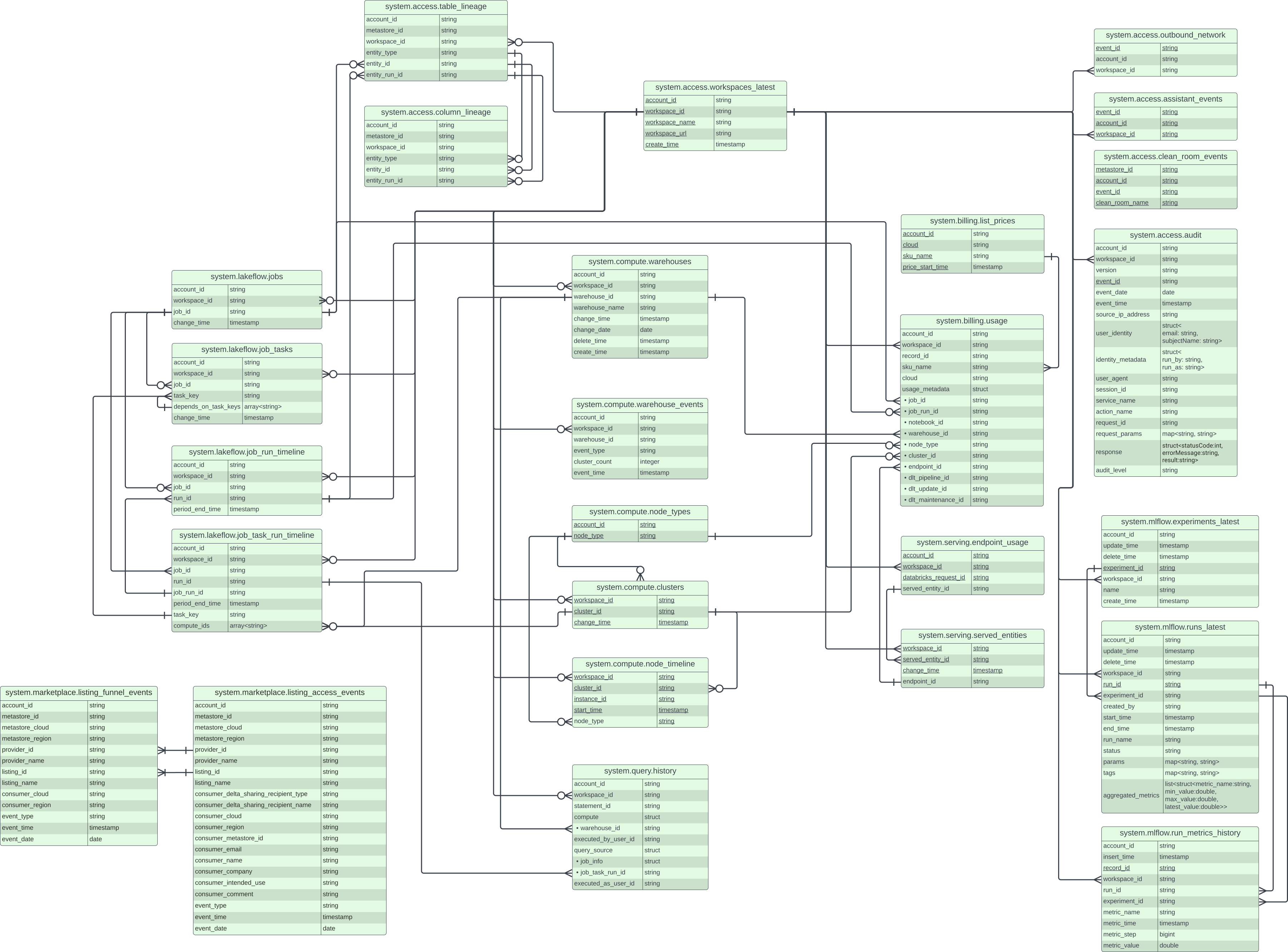
Source: Databricks

The lineage graph shows relationships between system tables across compute, billing, access, and query schemas. This is the starting point for building the context layer: understanding which tables exist and how they connect before documenting them.

The three business questions were chosen to represent real analyst needs around Databricks cost management, each requiring different table combinations and join logic. Correct answers to all three are immediately actionable for a data platform team.

Value-creation process:

Preparing the recipe components for the LLM to build the right context layer

Gather your PDFs / Images containing documentation about your data platform, its metadata/table, and column descriptions. In our case, it is the Databricks System tables lineage graph. Source: Databricks
We need to convert the PDF documentation into a YAML file. This can be done in multiple ways. We did it using the Mistral AI OCR model.
We get a yaml file showing the relations between the tables.
Human-in-the-loop: verify the generated YAML files.
Append the newly created yaml files (knowledge) into your Code Editor or into any Chat interface that supports knowledge collections
Enable data analysts to interact and use the knowledge for the work.

This article focuses primarily on steps 5-6: which is where we evaluate our context layer and show its benefits.

Using DocumentAI to generate semantic model for any AI/LLM assistant

Diagram: visual summary of the value-creation end-to-end process.

Evaluation framework

For each of the three business questions, we structured the evaluation as follows.

Business Question: What does the business wants to know
Prompt: Each prompt consists of 2 parts:
1. Part 1: a system prompt explaining LLM's context, goals and its role. See an example of our system prompt in Appendix 4.
2. Part 2 is the actual business question. The difference between a prompt for LLM with no recipe and LLM with the recipe: the latter gets an extra sentence saying to use the recipe files, and we point it to the exact files.
Analysis: To evaluate the LLM quality of text-to-SQL, we copied the generated SQL by LLM’s with and without the recipe. We ran the code in our Databricks workspace environment using SQL Compute and the system tables of Xomnia. This section compares the code output based on 3 categories: Accuracy, Hallucinations and Actionability.
Conclusion: results summary and determining the winner

Appendix 1: SQL for Business Question 1 (with Context)

Business question 1. The SQL result of the LLM with the recipe

The full SQL generated by the enriched LLM for "list all workspaces that are currently running and never used" is shown below. The model generated all CTEs correctly. One minor manual adjustment was made to the date range filter after initial review.

        SQL
    
WITH workspace_activity AS (
  -- Get all active workspaces
  SELECT DISTINCT w.workspace_id,
         w.workspace_name,
         w.workspace_url,
         w.status
  FROM system.access.workspaces_latest w
  WHERE w.status = 'RUNNING'
),

-- Check for billing usage (any DBU consumption)
workspace_billing AS (
  SELECT DISTINCT workspace_id
  FROM system.billing.usage
  WHERE usage_start_time >= '2025-09-01'
    AND usage_start_time < '2025-10-01'
),

-- Check for query activity
workspace_queries AS (
  SELECT DISTINCT workspace_id
  FROM system.query.history
  WHERE date(start_time) >= '2025-09-01'
    AND date(start_time) < '2025-10-01'
),

-- Final query: workspaces with no activity
final_cte AS (
  SELECT
    wa.workspace_id,
    wa.workspace_name,
    wa.workspace_url,
    wa.status,
    ew.total_dbu_used,
    CASE
      WHEN wb.workspace_id IS NOT NULL THEN 'Has Billing'
      ELSE 'No Billing'
    END AS billing_status
  FROM workspace_activity wa
  LEFT JOIN workspace_billing wb ON wa.workspace_id = wb.workspace_id
  LEFT JOIN workspace_queries wq ON wa.workspace_id = wq.workspace_id
  WHERE wb.workspace_id IS NULL
    AND wq.workspace_id IS NULL
  ORDER BY wa.workspace_name
)

Appendix 2:SQL for Business Question 2 (with Context)

Business question 2. The SQL result of the LLM with the recipe

The full SQL for "costs per service type across the organisation, including distinct user counts" is below. The model used both billing and query history tables for user identification, which was technically valid but slightly over-engineered. The cost calculations were correct.

        SQL
    
WITH billing_with_pricing AS (
 -- Join usage data with pricing to calculate costs
 SELECT
   u.billing_origin_product,
   u.sku_name,
   u.usage_quantity,
   u.usage_unit,
   u.usage_date,
   u.workspace_id,
   u.identity_metadata,
   u.usage_metadata,
   -- Calculate cost using effective list price
   u.usage_quantity * COALESCE(
     p.pricing.promotional.default,
     p.pricing.effective_list.default,
     p.pricing.default
   ) as calculated_cost
 FROM system.billing.usage u
 LEFT JOIN system.billing.list_prices p
   ON u.sku_name = p.sku_name
   AND u.cloud = p.cloud
   AND u.usage_date >= DATE(p.price_start_time)
   AND u.usage_date < COALESCE(DATE(p.price_end_time), '2099-12-31')
 WHERE u.usage_date >= '2025-09-01'
   AND u.usage_date <= '2025-10-31'
   AND u.record_type = 'ORIGINAL'
),

user_identification AS (
 -- Extract user identities from various sources
 SELECT DISTINCT
   billing_origin_product,
   sku_name,
   workspace_id,
   usage_date,
   calculated_cost,
   COALESCE(
     identity_metadata.run_as,
     identity_metadata.owned_by,
     identity_metadata.created_by
   ) as user_identity
 FROM billing_with_pricing
 WHERE COALESCE(
   identity_metadata.run_as,
   identity_metadata.owned_by,
   identity_metadata.created_by
 ) IS NOT NULL
),

-- Get additional users from query history for SQL-related usage
query_users AS (
 SELECT DISTINCT
   'SQL' as billing_origin_product,
   DATE(qh.start_time) as usage_date,
   qh.workspace_id,
   qh.executed_by as user_identity
 FROM system.query.history qh
 WHERE DATE(qh.start_time) >= '2025-09-01'
   AND DATE(qh.start_time) <= '2025-10-31'
   AND qh.executed_by IS NOT NULL
),

-- Get users from audit logs for broader coverage
audit_users AS (
 SELECT DISTINCT
   CASE
     WHEN a.service_name IN ('jobs', 'jobsService') THEN 'JOBS'
     WHEN a.service_name IN ('sql', 'sqlAnalytics') THEN 'SQL'
     WHEN a.service_name IN ('notebook', 'notebooks') THEN 'INTERACTIVE'
     WHEN a.service_name IN ('mlflow', 'modelServing') THEN 'MODEL_SERVING'
     WHEN a.service_name IN ('unityCatalog', 'catalog') THEN 'MANAGED_STORAGE'
     ELSE 'OTHER'
   END as billing_origin_product,
   a.event_date as usage_date,
   a.workspace_id,
   COALESCE(
     a.user_identity.email,
     a.identity_metadata.run_as,
     a.identity_metadata.run_by
   ) as user_identity
 FROM system.access.audit a
 WHERE a.event_date >= '2025-09-01'
   AND a.event_date <= '2025-10-31'
   AND COALESCE(
     a.user_identity.email,
     a.identity_metadata.run_as,
     a.identity_metadata.run_by
   ) IS NOT NULL
),

-- Combine all user sources
all_users AS (
 SELECT billing_origin_product, usage_date, workspace_id, user_identity
 FROM user_identification
  UNION ALL
  SELECT billing_origin_product, usage_date, workspace_id, user_identity
 FROM query_users
  UNION ALL
  SELECT billing_origin_product, usage_date, workspace_id, user_identity
 FROM audit_users
),

-- Aggregate costs by product
product_costs AS (
 SELECT
   billing_origin_product,
   SUM(calculated_cost) as total_cost
 FROM billing_with_pricing
 GROUP BY billing_origin_product
),

-- Count distinct users by product
product_users AS (
 SELECT
   billing_origin_product,
   COUNT(DISTINCT user_identity) as distinct_users
 FROM all_users
 GROUP BY billing_origin_product
)

-- Final result combining costs and user counts
SELECT
 COALESCE(pc.billing_origin_product, pu.billing_origin_product) as product_name,
 ROUND(COALESCE(pc.total_cost, 0), 2) as cost,
 COALESCE(pu.distinct_users, 0) as number_of_distinct_users,
  CASE
   WHEN COALESCE(pu.distinct_users, 0) > 0
   THEN ROUND(COALESCE(pc.total_cost, 0) / pu.distinct_users, 2)
   ELSE 0
 END as cost_per_user,
  CASE
   WHEN COALESCE(pc.billing_origin_product, pu.billing_origin_product) IN ('JOBS', 'DLT')
     THEN 'Data Processing'
   WHEN COALESCE(pc.billing_origin_product, pu.billing_origin_product) IN ('SQL', 'INTERACTIVE', 'ALL_PURPOSE')
     THEN 'Analytics & Development'
   WHEN COALESCE(pc.billing_origin_product, pu.billing_origin_product) IN ('MODEL_SERVING', 'VECTOR_SEARCH', 'LAKEHOUSE_MONITORING')
     THEN 'ML & AI Services'
   WHEN COALESCE(pc.billing_origin_product, pu.billing_origin_product) IN ('MANAGED_STORAGE', 'FINE_GRAINED_ACCESS_CONTROL')
     THEN 'Data Management'
   WHEN COALESCE(pc.billing_origin_product, pu.billing_origin_product) IN ('NETWORKING', 'SHARED_SERVERLESS_COMPUTE')
     THEN 'Infrastructure'
   WHEN COALESCE(pc.billing_origin_product, pu.billing_origin_product) IN ('APPS', 'BASE_ENVIRONMENTS')
     THEN 'Application Platform'
   ELSE 'Other Services'
 END as product_category

FROM product_costs pc
FULL OUTER JOIN product_users pu
 ON pc.billing_origin_product = pu.billing_origin_product

ORDER BY cost DESC, number_of_distinct_users DESC;

Appendix 3: SQL for Business Question 3 (with Context)

The full SQL for "all compute resources with their auto-termination settings, filtering for those with no auto-stop or settings above 45 minutes" is below. The key contribution of The Context here was the inclusion of delete_time, which changed the actionability of the entire output.

Business question 3. The SQL result of the LLM with the recipe

        SQL
    
-- Complete inventory of all Databricks compute resources with auto-termination settings
-- Covers SQL Warehouses and Clusters for September-October 2025
-- Improved version using CTEs and better SQL practices

WITH date_filter AS (
 SELECT
   DATE('2025-09-01') as start_date,
   DATE('2025-10-30') as end_date
),

warehouse_settings AS (
 SELECT
   'SQL_WAREHOUSE' as resource_type,
   warehouse_id as resource_id,
   warehouse_name as resource_name,
   workspace_id,
   warehouse_type as resource_subtype,
   warehouse_size as size_configuration,
   auto_stop_minutes,
   CASE
     WHEN auto_stop_minutes IS NULL THEN 'NO_AUTO_STOP'
     WHEN auto_stop_minutes > 45 THEN 'LONG_AUTO_STOP'
     ELSE 'ACCEPTABLE_AUTO_STOP'
   END as auto_stop_status,
   CONCAT('Min: ', COALESCE(min_clusters, 0), ', Max: ', COALESCE(max_clusters, 0)) as scaling_config,
   'System' as owner,
   change_time as last_modified,
   delete_time
 FROM system.compute.warehouses w
 CROSS JOIN date_filter df
 WHERE w.change_time >= df.start_date
   AND (w.delete_time IS NULL OR w.delete_time >= df.start_date)
),

cluster_settings AS (
 SELECT
   CASE
     WHEN cluster_source = 'JOB' THEN 'JOB_CLUSTER'
     WHEN cluster_source IN ('PIPELINE', 'PIPELINE_MAINTENANCE') THEN 'PIPELINE_CLUSTER'
     ELSE 'ALL_PURPOSE_CLUSTER'
   END as resource_type,
   cluster_id as resource_id,
   COALESCE(cluster_name, 'Unnamed Cluster') as resource_name,
   workspace_id,
   cluster_source as resource_subtype,
   CONCAT(
     COALESCE(driver_node_type, 'Unknown'), ' (driver), ',
     COALESCE(worker_node_type, 'Unknown'), ' (worker)'
   ) as size_configuration,
   auto_termination_minutes as auto_stop_minutes,
   CASE
     WHEN auto_termination_minutes IS NULL THEN 'NO_AUTO_TERMINATION'
     WHEN auto_termination_minutes > 45 THEN 'LONG_AUTO_TERMINATION'
     ELSE 'ACCEPTABLE_AUTO_TERMINATION'
   END as auto_stop_status,
   CASE
     WHEN worker_count IS NOT NULL THEN CONCAT('Fixed: ', worker_count, ' workers')
     WHEN min_autoscale_workers IS NOT NULL AND max_autoscale_workers IS NOT NULL
       THEN CONCAT('Auto: ', min_autoscale_workers, '-', max_autoscale_workers, ' workers')
     ELSE 'Single node'
   END as scaling_config,
   COALESCE(owned_by, 'Unknown') as owner,
   change_time as last_modified,
   delete_time
 FROM system.compute.clusters c
 CROSS JOIN date_filter df
 WHERE c.change_time >= df.start_date
   AND (c.delete_time IS NULL OR c.delete_time >= df.start_date)
),

combined_resources AS (
 SELECT * FROM warehouse_settings
 UNION ALL
 SELECT * FROM cluster_settings
)

SELECT
 resource_type,
 resource_id,
 resource_name,
 workspace_id,
 resource_subtype,
 size_configuration,
 auto_stop_minutes,
 auto_stop_status,
 scaling_config,
 owner,
 last_modified,
 delete_time,
 -- Additional computed fields for analysis
 CASE
   WHEN delete_time IS NOT NULL THEN 'DELETED'
   WHEN auto_stop_minutes IS NULL THEN 'NEEDS_CONFIGURATION'
   WHEN auto_stop_minutes > 45 THEN 'NEEDS_OPTIMIZATION'
   ELSE 'PROPERLY_CONFIGURED'
 END as configuration_status
FROM combined_resources
ORDER BY
 resource_type,
 workspace_id,
 CASE WHEN auto_stop_minutes IS NULL THEN 0 ELSE auto_stop_minutes END DESC,
 resource_name;

Appendix 4

System prompt for all 3 Business questions, used for both the LLM with and without the recipe

Goal: Shape analysis of the usage of Databricks internally

How: produce analytics queries in SQL for the data platform observability team

Context: Generate queries that can be used by the team to better understand the usage of Databricks internally

Source: official databricks documentation page of system tables: https://docs.databricks.com/aws/en/admin/system-tables/ *

Data source: system tables in databricks

Data timeline: September 2025

---

META DESCRIPTION (155 chars):

We ran the same text-to-SQL queries through an LLM with and without a semantic layer on Databricks system tables. Here is what happened and what it means for your analytics team.

PULL QUOTE:

"Context does not guarantee perfect analytical depth. It prevents errors. And you cannot iterate on a query that will not run."

Written by

Maksi Melnikov

Analytics Engineer at Xomnia.

Technology

SQL

Topic

Analytics Engineering

Data Platforms